5.2 Water Balance Impacts

Water balance components like soil moisture, precipitation, and runoff can vary greatly across spatial and temporal scales. This makes comprehensive measurements challenging and expensive. In order to understand and model such components accurately and efficiently, field campaigns and experiments should be designed to collect appropriate data types and amounts, and allow scaling across time and space. Accurate measurements also greatly help in effective management of water resources.

In this section you will:

• use tested methodologies to efficiently scale point measurement up to the spatial extent of interest.

• learn how CZ processes and land management decisions impact the water balance. The process of decision-making for water resources requires deep understanding of the water cycle and quantitative data to best balance both societal and environmental water needs.

Scaling of Point Measurements

Scientists use data from multiple rain gages to estimate the rainfall distribution over an area. The distribution may be for specific storms, days, months, or even years. It may be necessary to determine an average depth or a spatial distribution of depths.

Precipitation is highly variable. When multiple gauges area available, the spatial average precipitation must be calculated from point measurements.  A weighed average approach is commonly used:

(2)\[\begin{split}\begin{align} P &= \sum_{i=1}^n w_i P_i\\ \sum_{i=1}^n w_i &= 1 \end{align}\end{split}\]

where \(P\) is the precipitation measured at a gauge (\(i\)), \(n\) is the total number of gauges, and \(w\) is the weight assigned to a gauge. Most common approaches to estimate spatial average of multiple gauges are simply methods to assign weights. For example, we could elect to simply take the direct average of all of our gauges. In this case, each gauge gets an equal weight. If \(n = 3\), each gauge gets a weight of 1/3. This is the same as same as simply adding up each \(P\) and dividing by the number of gauges.

A problem with the direct averaging approach is it assumes that the gauges are placed in a way that captures the actual spatial variability. For example, we know that in mountainous terrain precipitation tends to be higher at higher elevations in a watershed. If all of our gauges are placed at high elevations, we will overestimate the average. If the gauges, however, are placed throughout the watershed in a way that appropriately represents the relationship between precipitation and elevation, our direct average will be more accurate.

If the rain gages are evenly distributed, a simple arithmetic average will be adequate. If the gages are not evenly distributed, other methods have to be considered.

Thiessen Polygon Method

One of the most widely used methods to calculate aerial precipitation is the Thiessen polygon method. The use of the Thiessen polygon method is illustrated in Fig. 36. The locations of each rain gage in and immediately adjacent to the area of interest are located on a map. The rainfall amount at each gage is noted. The straight dashed lines are drawn between each adjacent gage site; then, solid perpendicular bisectors to these lines are constructed so that the area around each gage is enclosed by the bisectors or the area boundary. The enclosed areas around each gage are known as Thiessen polygons. The entire area within each polygon is closer to the rain gage in that polygon than to any other rain gage. The rainfall amount measured by the gage within each polygon is assumed to be representative of the rainfall for that polygon. The areas of each polygon are calculated by geometry, with a planimeter, with graph paper, or with a computer-aided drawing package. The average rainfall for the entire area is then assumed to be a weighted average of the observed rainfalls, as shown below:

(3)\[P = \dfrac{\sum_{i=1}^n A_i P_i}{\sum_{i=1}^n A_i}\]

where \(P\) represents the average depth of rainfall in the watershed with a total area of \(\sum_{i=1}^n A_i\), and \(A_i\) is the area of the \(i\)th polygon with precipitation of \(P_i\) in that polygon.

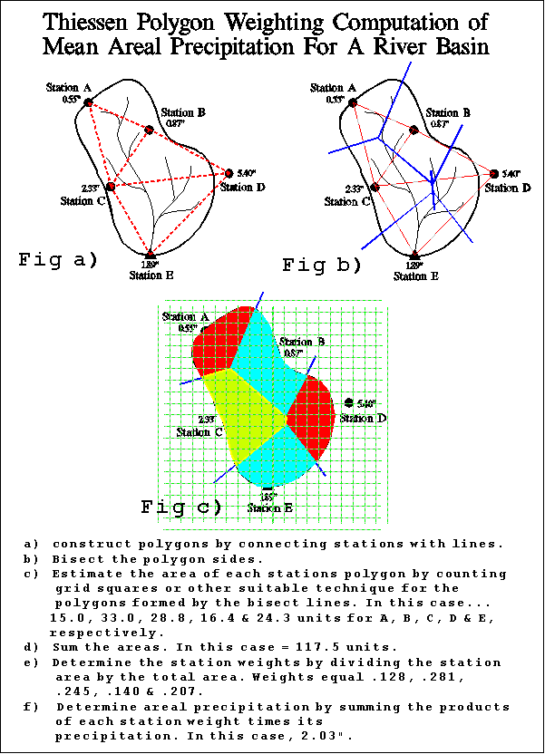
Fig. 36 This graphical technique calculates station weights based on the relative areas of each measurement station in the Thiessen polygon network. The individual weights are multiplied by the station observation and the values are summed to obtain the areal average precipitation.

Image source: Precipitation Measurements (weather.gov)

Thiessen Polygon Interpolation

Here are the steps involved in Thiessen Polygon Interpolation:

• Identify Known Points: Start with known values in your dataset.

• Constructing Thiessen Polygons:

  • Starting Point: Begin with a set of discrete sample points on a plane. These could be locations of weather stations, archaeological sites, or any other point data.

  • Drawing Perpendicular Bisectors: For every pair of neighboring points, draw the perpendicular bisector (a line that cuts in half the shortest distance between them). This bisector represents a boundary where locations are equidistant to the two points.

  • Meeting of Bisectors: As more bisectors are drawn, they’ll intersect, forming the vertices of polygons.Completing the Polygon: Once all necessary bisectors have been drawn, the polygons are formed, each surrounding its respective sample point.

• Key Features and Assumptions: Each polygon represents the region of influence of its central sample point. Any location inside a particular Thiessen polygon is closer to its central sample point (or “source point”) than to any other sample point outside the polygon.

• Interpolate: Finally, use the value of the central point of each Thiessen polygon to estimate values at unknown locations.

Example of Thiessen Polygon Interpolation

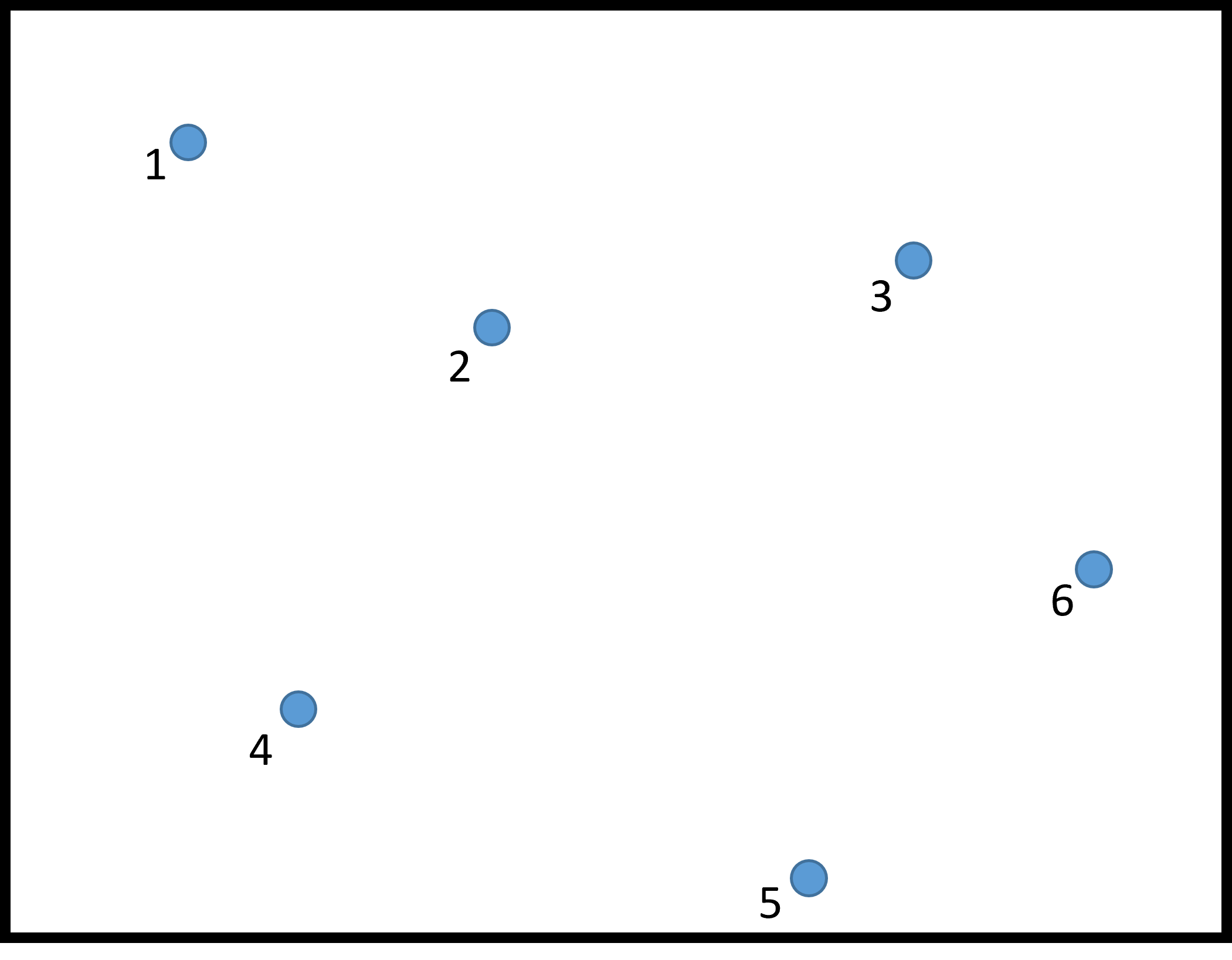
In the following watershed area, there are six meteorological stations where annual precipitation values are reported.

Met Station	Precipitation, mm
1	985
2	1015
3	963
4	1101
5	1057
6	1078

Calculate the annual precipitation for the entire area.

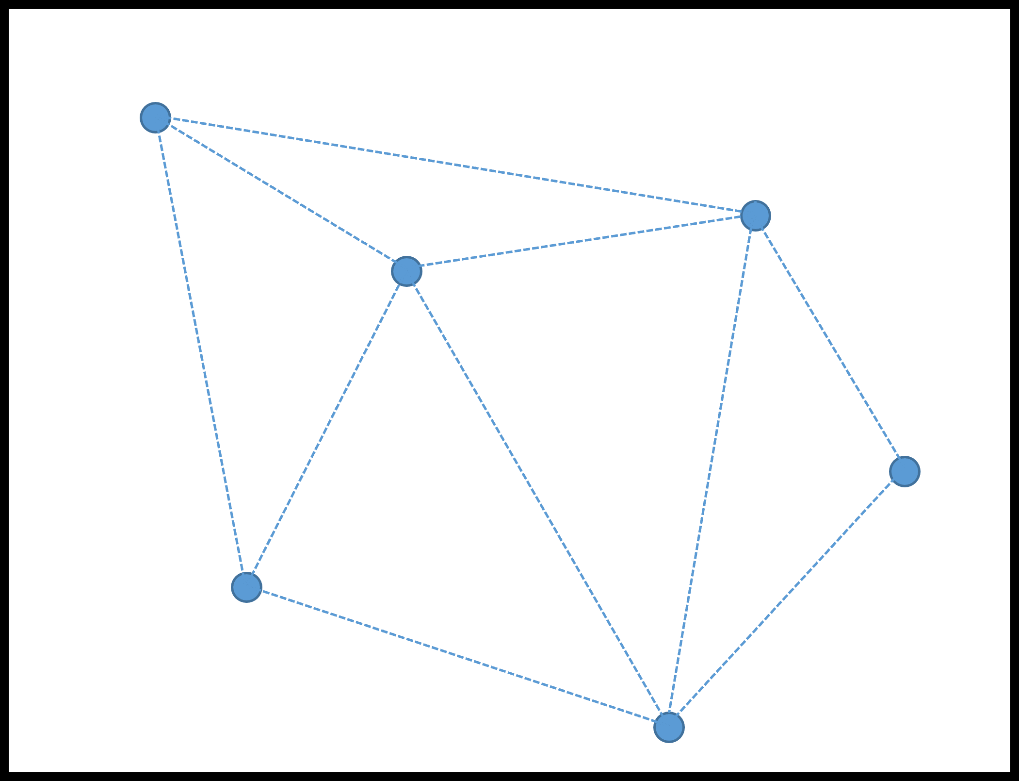
• Step 1: Draw lines connecting all the points to their two nearest neighbors.

• Step 2: Draw lines that bisect (divide the lines in half) perpendicular to the lines connecting the points.

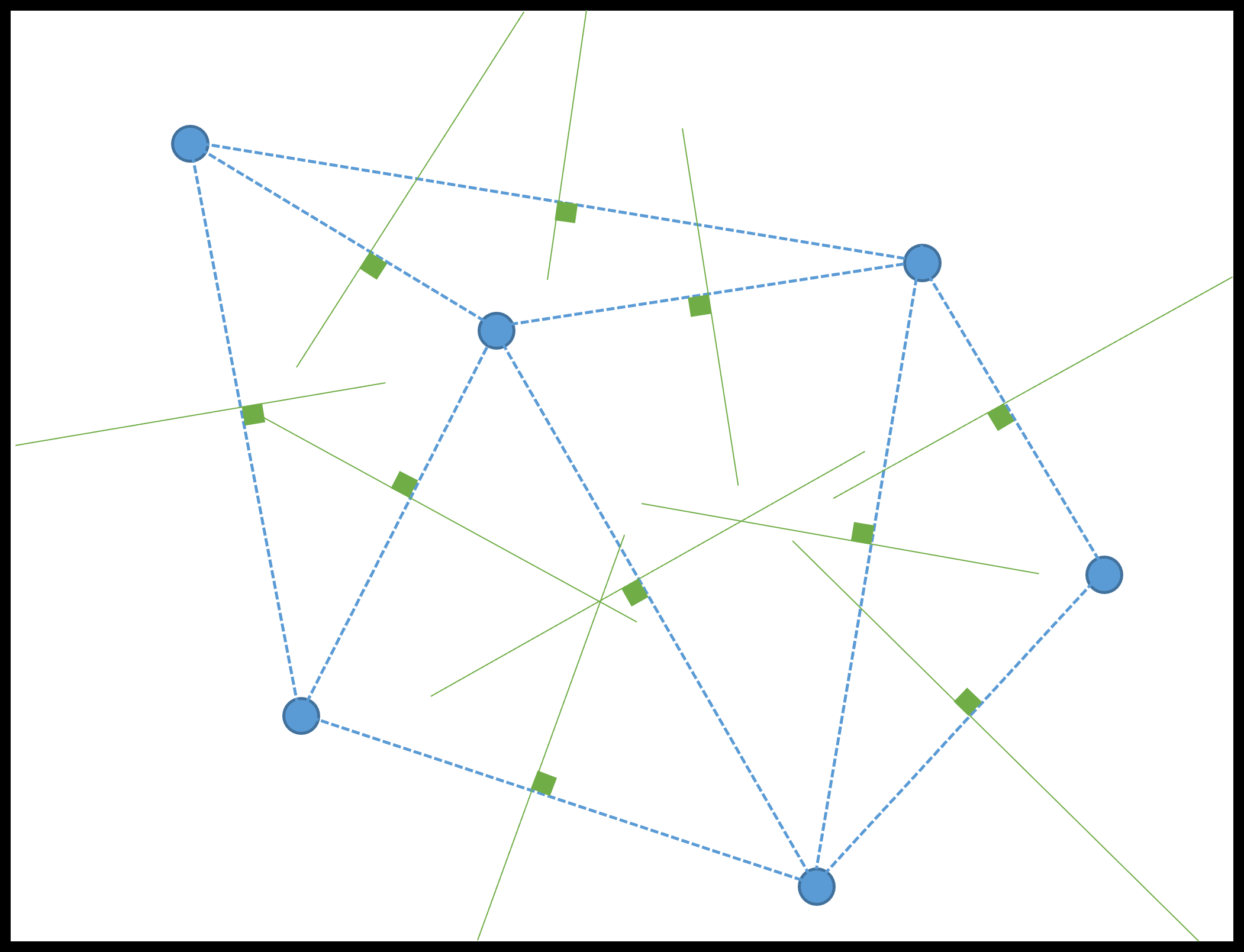
• Step 3: Lengthen or shorten all lines to make them connect. Note that they should all come to a single point.

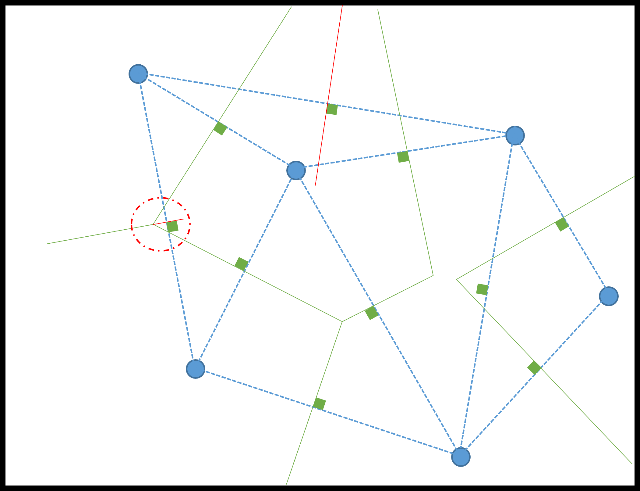
• Step 4: Remove all the unnecessary lines.

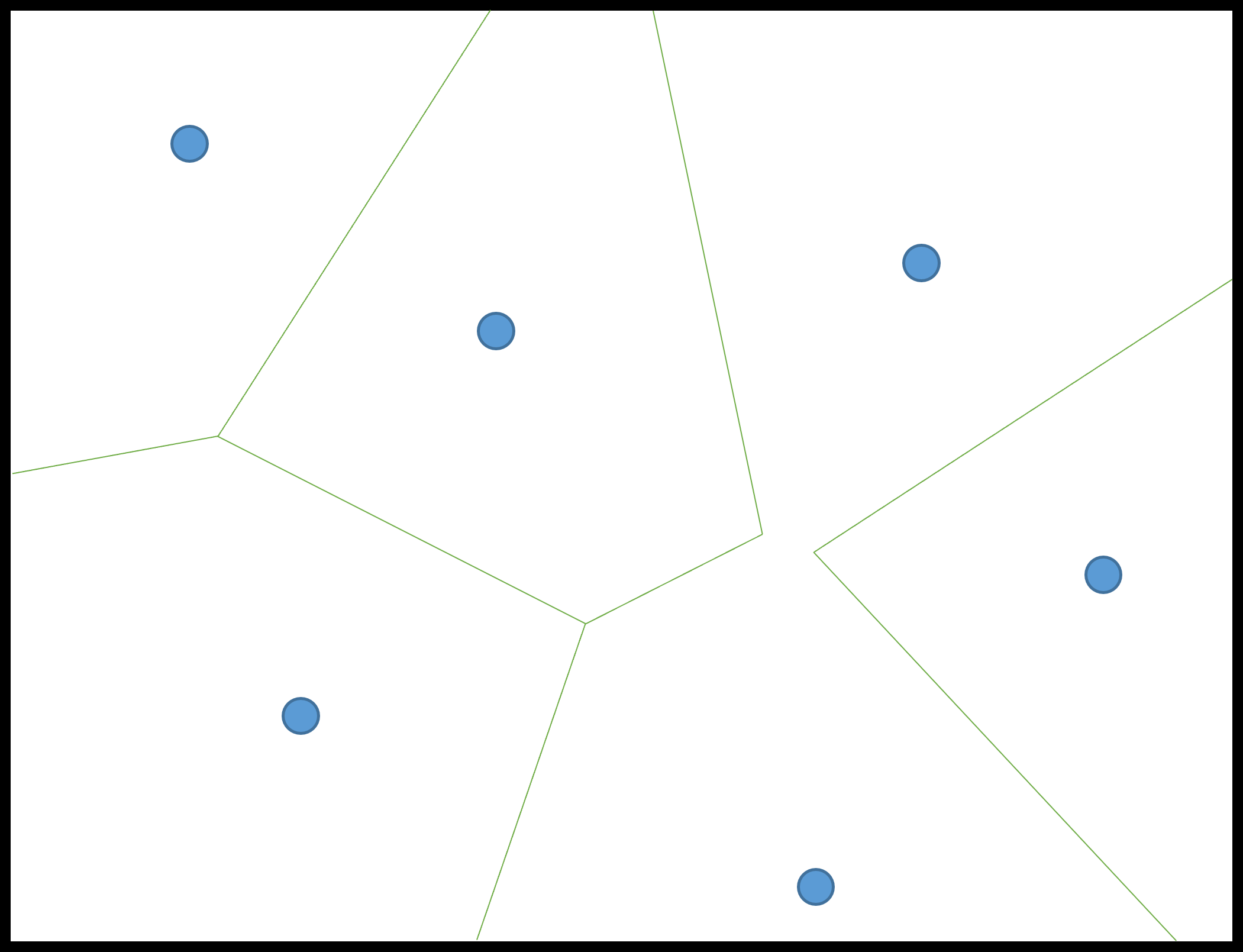
• Step 5: Once the final image is obtained, the proportions of each polygon to the whole should be calculated. This can be performed using geometry or by printing the Thiessen polygons on graph paper and counting the boxes in each polygon.

\[ \% \text{Area} = \frac{\text{# of Pixels in polygon }}{\text{# of Pixels in Extent}} \times 100\% \]

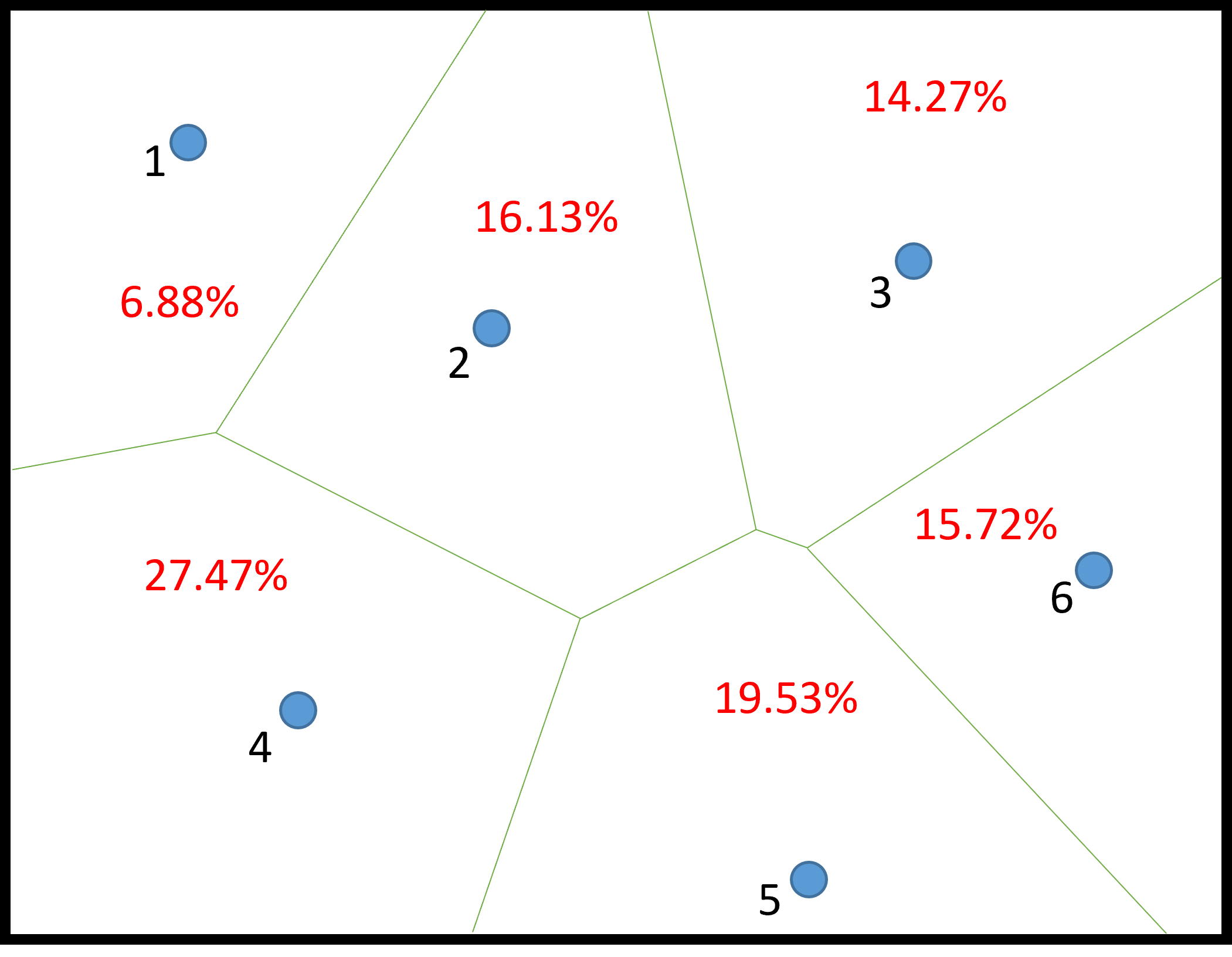
• Step 6: Calculate the weighted precipitation value for the area around each met station

\[ P_\text{area} = P_\text{Met Station} \times \text{Area} \]

• Step 7: Calculate the weighted precipitation for the entire extent

\[ P_\text{Basin} = \sum (P_\text{Met Station} \times \text{Area}) \]

Setting all the calculations in a table, we can see that the precipitation for the entire basin is \(\pu{1047.2 mm} \)

Met Station	Precip. (mm)	% Area	Weighted Precip. (mm)
1	985	6.9	68
2	1015	16.1	163.4
3	963	14.3	137.7
4	1101	27.5	302.8
5	1057	19.5	206.1
6	1078	15.7	169.3
		Sum	1047.2

Inverse Distance Weighted Method

Inverse distance weighted (IDW) interpolation explicitly makes the assumption that things that are close to one another are more alike than those that are farther apart. To predict a value for any unmeasured location, IDW uses the measured values surrounding the prediction location. The measured values closest to the prediction location have more influence on the predicted value than those farther away. IDW assumes that each measured point has a local influence that diminishes with distance. It gives greater weights to points closest to the prediction location, and the weights diminish as a function of distance, hence the name inverse distance weighted. It is calculated as shown below.

(4)\[P=\dfrac{\sum_{i=1}^n (\dfrac{P_i}{d_i} )}{\sum_{i=1}^n (\dfrac{1}{d_i})}\]

where \(P\) represents the average depth of rainfall in the watershed and \(d_i\) is the distance from a known point.

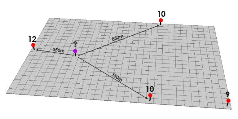
Fig. 37 Interpolation between three known values involves identifying the closest neighbor or centroid between the three values that best captures the

Image source: Inverse Distance Weighting (IDW) Interpolation - GIS Geography

Inverse Distance Weighting (IDW)

Here are the steps involved in Inverse Distance Weighting (IDW):

• Identify Known Points: Start with known values in your dataset.

• Spatial Autocorrelation: IDW assumes that things that are close to one another are more alike than those that are farther apart. This is known as spatial autocorrelation.

• Calculate Path Distances: Calculate path distances from each known point to each prediction point.

• Assign Weights: Assign weights to the known points based on their distance from the prediction location. The closer a known point is to the prediction location, the more influence it has on the predicted value.

Example of IDW Interpolation

In the following watershed area (same as the Thiessen Polygon Method example), there are six meteorological stations where annual precipitation values are reported.

Met Station	Precipitation, mm
1	985
2	1015
3	963
4	1101
5	1057
6	1078

Calculate the annual precipitation for the entire area.

• Step 1: Decide how many pixels to create. Let us choose six for this example. There will come a point where adding pixels will not improve the result.

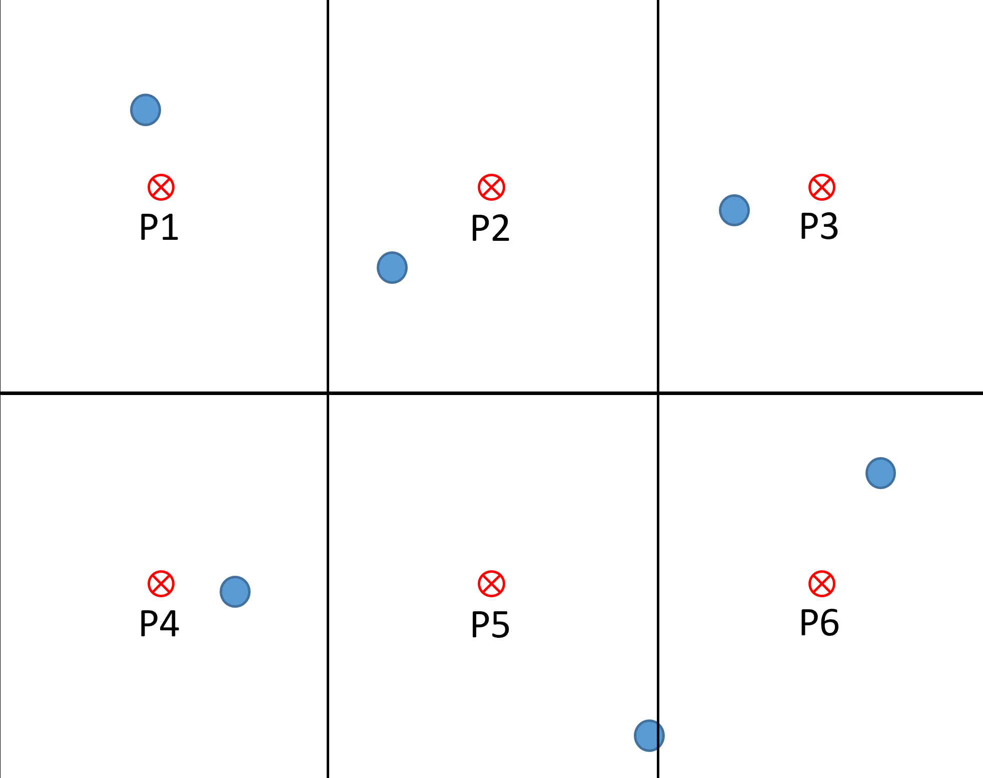
• Step 2: Choose the nearest three neighbors to each centroid in a pixel.

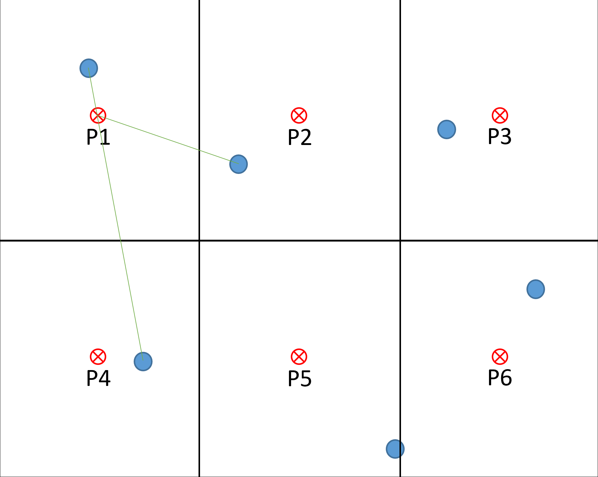
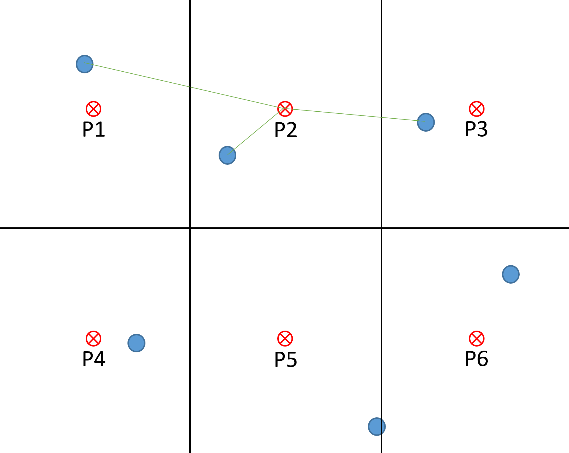
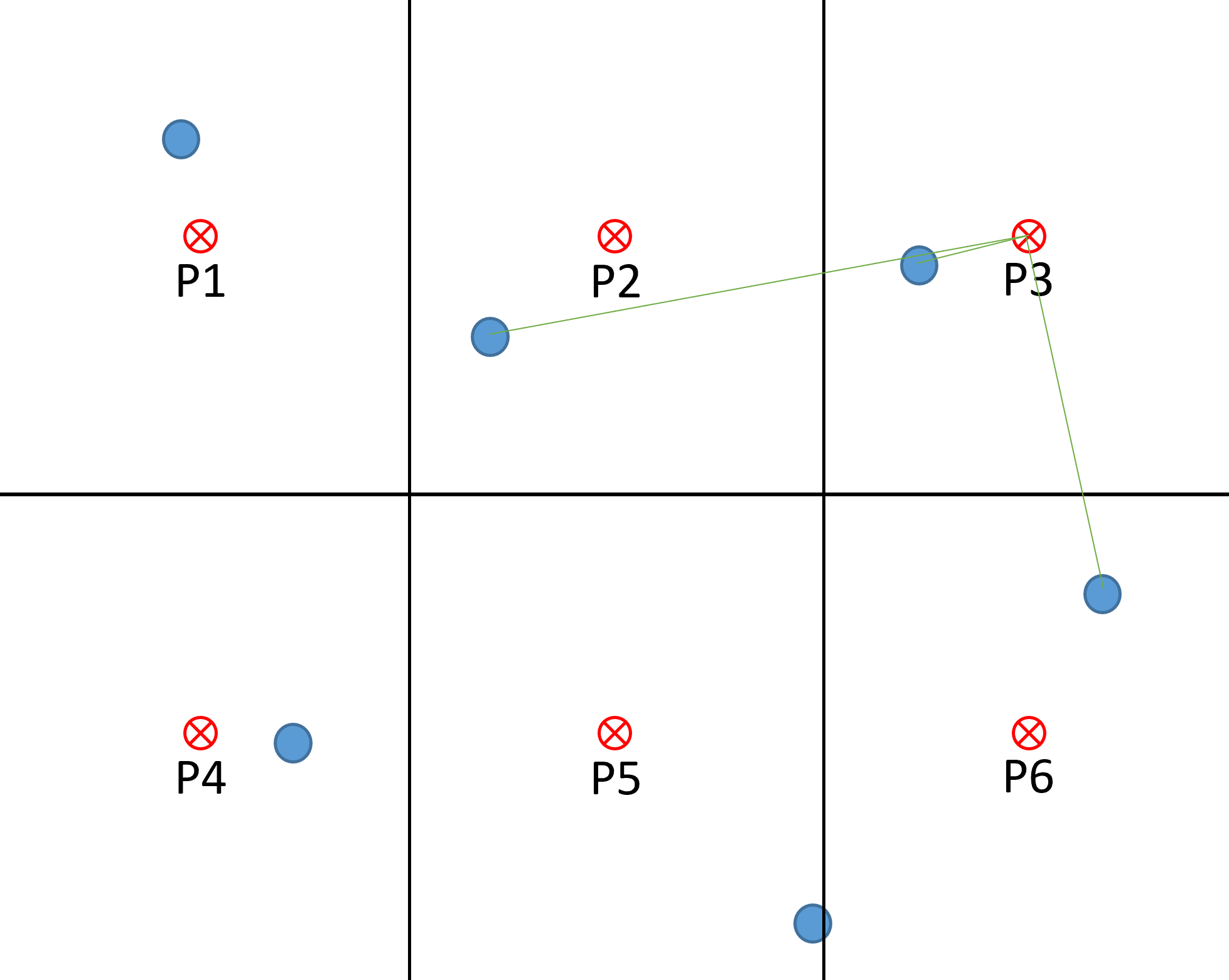
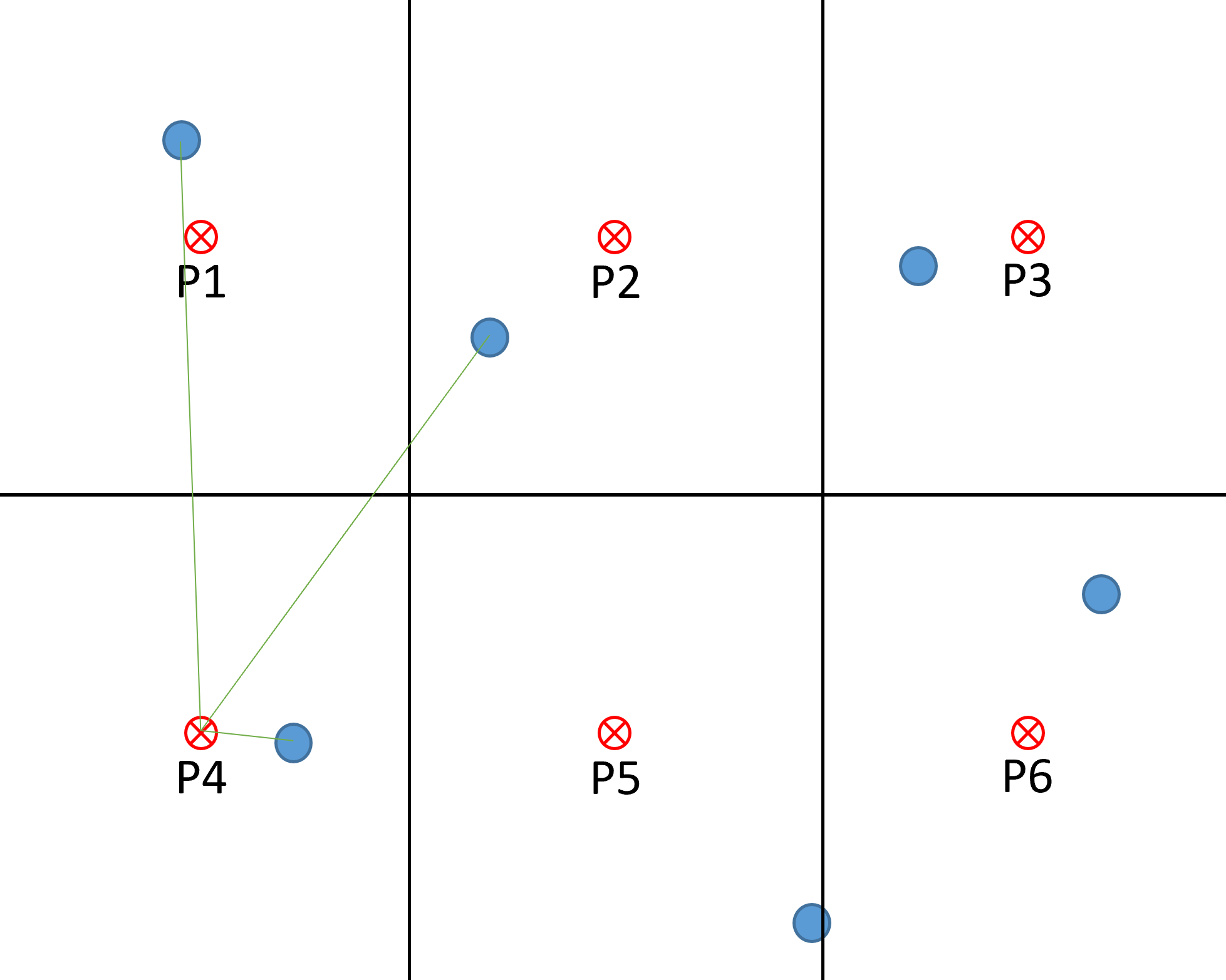
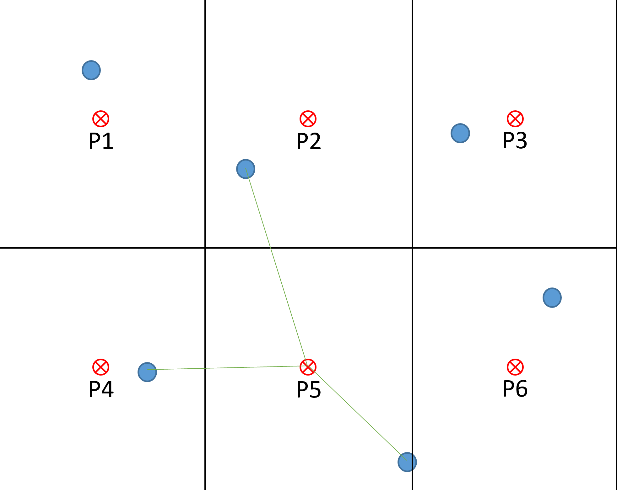
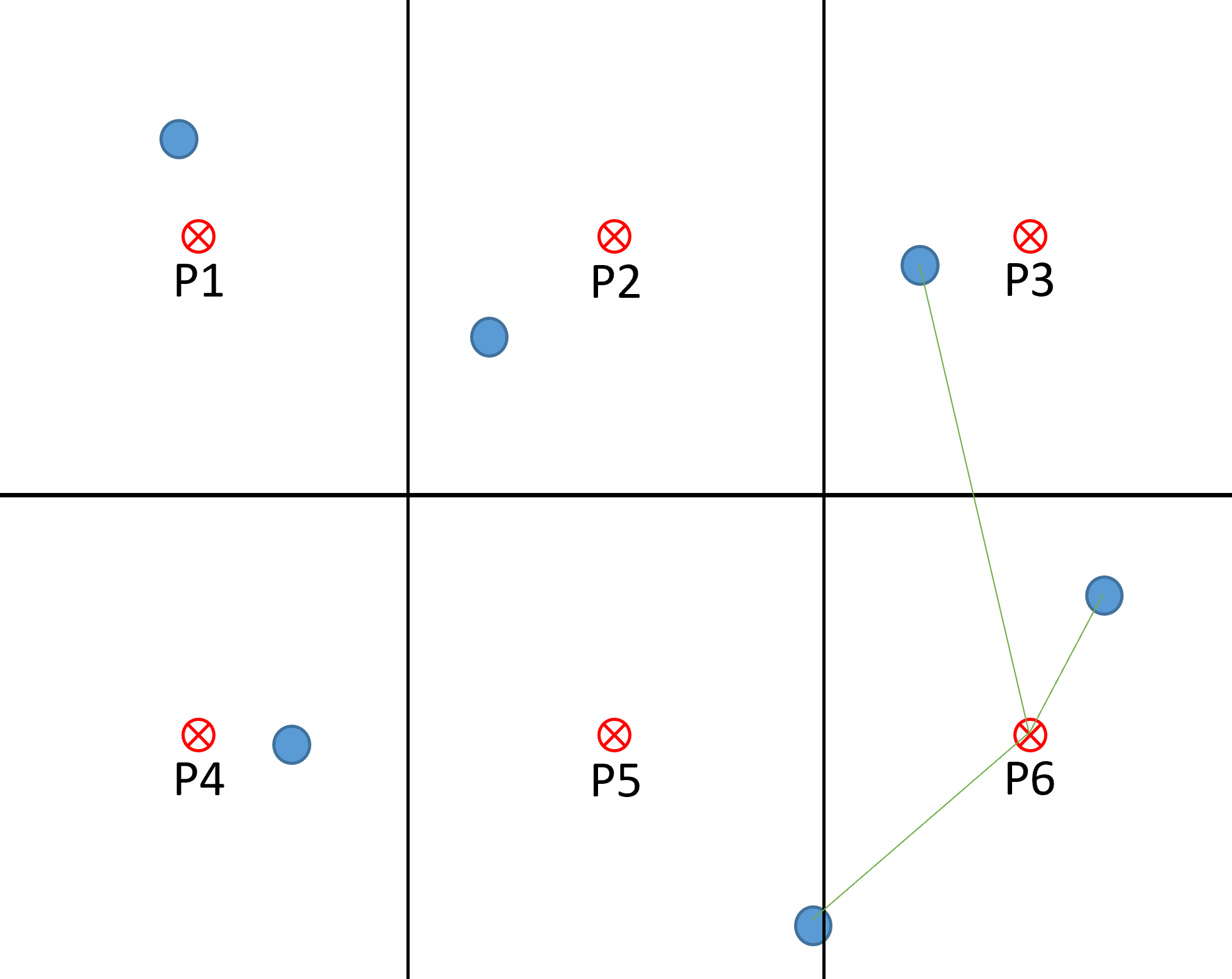
• Step 3: Calculate the IDWs for each pixel as follows.

(5)\[\begin{eqnarray} P_{extent} &=& \dfrac{\sum (w_i \times P_{annual})}{\sum w_i}\\ \text{where,}\ w_i &=& \frac{1}{\text{distance}_i} \end{eqnarray}\]

For Pixel 1: Example calculation for an upper left corner pixel using neighbors 1, 2, and 4:

(6)\[\begin{equation} \dfrac{\dfrac{1}{1.2}\times 985 + \dfrac{1}{3.8} \times 1015 + \dfrac{1}{6.4} \times 1101}{\dfrac{1}{1.2}+\dfrac{1}{3.8}+\dfrac{1}{6.4}} = \pu{1005.8 mm} \end{equation}\]

• Step 4: Calculate IDWs for all pixels

Setting all the calculations in a table, we can see that the precipitation for the entire basin is \(\pu{1047.2 mm} \)

Pixel #	Nearest Met Stations	Distance (cm)	Annual Precip (mm)	Pixel Annual Precip (mm)
1	1, 2, 4	1.2, 3.8, 6.4	985, 1015, 1101	1005.8
2	1, 2, 3	5.5, 2.0, 3.8	985, 1015, 963	994.8
3	2, 3, 6	6.8, 1.4, 4.5	1015, 963, 1078	993.6
4	1, 2, 4	6.3, 5.5, 1.3	985, 1015, 1101	1070.3
5	2, 4, 5	5.1, 4.0, 3.4	1015, 1101, 1057	1060.7
6	3, 5, 6	5.9, 3.5, 1.9	963, 1057, 1078	1052.0

• Step 5: Calculate weighted precip for entire basin. Since the six pixels are equal size, just need to take arithmetic mean.

\[ \text{Weighted Precip} = \frac{1005.8+994.8+993.6+1070.3+1060.7+1052.0}{6} = \pu{1029.5 mm} \]

This final value is similar to the value obtained using the Thiessen Polygon Method - a difference of less than 2%.

Hypsometric Method

The term hypsometry refers to the measurement of elevation. The hypsometric method combines the distribution of elevation within a watershed with a known relationship between precipitation and elevation to determine weights for elevation classes. An advantage of the hypsometric method in mountainous terrain is that is accounts for the mechanism that is known to produce spatial variability of precipitation.

The method combines the distribution of elevation within a watershed with a knowledge of the precipitation-elevation relationship to determine weights for elevation classes. These weights are then used to calculate the average precipitation over the watershed.

The hypsometric method is a useful tool for estimating precipitation in mountainous areas, where the relationship between precipitation and elevation is often non-linear. The method is also relatively simple to implement, making it a good choice for watershed-scale studies.

Hypsometric Weighting Method

To calculate aerial precipitation using the hypsometric method, the following steps are taken:

• The distribution of elevation within the watershed is obtained. This can be done using a variety of methods, such as topographic maps, DEMs, or GPS data.

• The precipitation-elevation relationship is obtained. This can be done using historical data, climate models, or theoretical relationships.

• The weights for each elevation class are calculated. This is done by multiplying the area of each elevation class by the precipitation-elevation relationship for that elevation class.

• The average precipitation over the watershed is calculated by weighting the precipitation for each elevation class by the weights for that elevation class.

The method is relatively simple to implement and can be used to calculate average precipitation over large areas.

Water Management and Balance

Climate change is intensifying the water cycle to speed up as warming global temperatures increase the rate of evaporation worldwide. Increased evaporation in one part of the Earth system results in increased precipitation elsewhere. Extreme weather events are also causing extreme water scarcity, extreme precipitation, and degraded water environments. These impacts throughout the water cycle threaten sustainable development, biodiversity, and people’s access to water and sanitation.

According to the latest IPCC Assessment Report, managing water resources is very high on adaptation strategies.

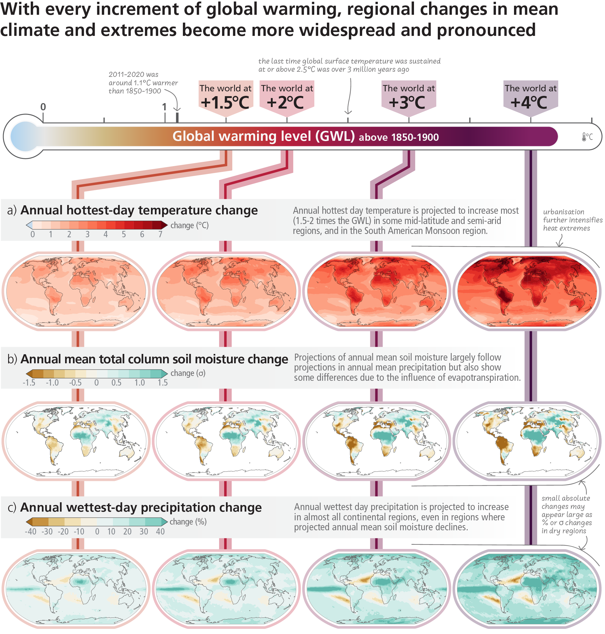
Fig. 38 Projected changes of annual maximum daily maximum temperature, annual mean total column soil moisture and annual maximum 1-day precipitation at global warming levels of 1.5°C, 2°C, 3°C, and 4°C relative to 1850–1900. Projected (a) annual maximum daily temperature change (°C), (b) annual mean total column soil moisture (standard deviation), (c) annual maximum 1-day precipitation change (%). The panels show CMIP6 multi-model median changes. In panels (b) and (c), large positive relative changes in dry regions may correspond to small absolute changes. In panel (b), the unit is the standard deviation of interannual variability in soil moisture during 1850–1900. Standard deviation is a widely used metric in characterising drought severity. A projected reduction in mean soil moisture by one standard deviation corresponds to soil moisture conditions typical of droughts that occurred about once every six years during 1850–1900.

Image source: Figures: AR6 Synthesis Report (ipcc.ch)

In many parts of the western United States, mountains can serve as “water towers”. However societal demand for water in the mountains is relatively lower. In California, precipitation falls in mountain ranges and flows via rivers and man-made aqueducts and canals to the areas where higher demand is located. Snowpack also acts as a reservoir, gradually releasing water downstream as it melts.

Much of California experiences a rainy season in the winter and spring, and a dry season in the summer and early fall. It is naturally driest during the peak of the agricultural growing season, when water demand is greatest. Residential and commercial areas also generally do not adjust their demands to follow the natural supply. To address this, there are large reservoirs to store winter precipitation and snowmelt. These reservoirs and their releases control the downstream flow in streams and rivers.

Land development can also have a significant impact on the water balance. Change in land use/cover impacts the water balance of a watershed by changing the magnitude and pattern of different components of the water balance resulting in increasing water management problem (e.g., Schilling et al., 2008,Kundu et al, 2017).

Due to the increased water stress, wildfires are expected to increase as well. Wildfires release ash and contaminants associated with ash into streams, lakes and water reservoirs. Vegetation that holds soil in place and retains water is burned away leading to other geological hazards. According to EPA, in the aftermath of a large wildfire, rainstorms flush vast quantities of ash, sediment, nutrients and contaminants into streams, rivers, and downstream reservoirs. Fire suppression in western U.S. mountains has caused dense forests with high evapotranspiration leading to heightened risk of wildfires. Restoring natural wildfire regimes to these forests could affect hydrology by changing vegetation composition and structure, but the specific effects on water balance are unknown (Boisramé et al., 2019).

Fire suppression can have a significant impact on water. Fire suppression runoff can contaminate soil and water with toxic or hazardous materials, and direct exposure to soil and water from hazardous materials whose containers/containment systems may fail due to fire. This can lead to contamination of the air via the fire plume and its subsequent diffusion, with deposition of particulate and other materials likely to contaminate soil and water (Martin et al., 2016).

Mini-Project #6

Part A

Read Mountain runoff vulnerability to increased evapotranspiration with vegetation expansion

Cooperatively and collaboratively present the main findings from this paper for the Southern Sierra Nevada CZO.  See the below breakdown of tasks for the format. Use good screenshots of the figures and graphs and add text.

Add your name to one part and take ownership of the appropriate slides. The Results and Discussion sections can be worked on with a partner.

1. Main goals, hypotheses, and objectives

2. Site information - include maps

3. Methods - summary w/ representative pictures of methods

4. Main Results - select a few (not all)

5. Discussion of Data

6. Conclusions

Part B

Complete the SimWater exercise posted on OAKS.

Readings and resources for this section

1. Mountain runoff vulnerability to increased evapotranspiration with vegetation expansion | PNAS

2. Physical Hydrology, Third Edition, by S. Lawrence Dingman - See OAKS for Chapters 1 and 2.

3. Precipitation Measurements (weather.gov)