
6.1 Biogeochemistry in the CZ#
Biogeochemistry is the chemistry of the surface of the Earth. This chemistry is influenced by life on Earth and rapidly changing under the outsized influence of human actions.
Biogeochemical processes are essential for the functioning of the CZ. These processes include the cycling of nutrients, the production of \(\ce{O2}\), and the regulation of climate. Biogeochemical processes are also affected by human activity. For example, the burning of fossil fuels releases \(\ce{CO2}\) into the atmosphere, which can contribute to climate change.
Biogeochemistry is important for understanding how the critical zone is affected by human activity. This information can be used to develop sustainable management practices that protect the critical zone.
Here are some specific examples of how biogeochemistry is important for the critical zone:
Nutrients are essential for life, and they are cycled through the critical zone by biogeochemical processes.
Water is essential for life, and it is moved through the CZ.
Photosynthesis is a process that plants use to convert sunlight into energy. As a byproduct of photosynthesis, plants release oxygen into the atmosphere.
Human activities, such as agriculture, deforestation, and climate change, can affect biogeochemical processes. It is important to understand biogeochemistry in order to protect the critical zone. The critical zone is essential for life on Earth, and it is important to ensure that it is healthy and sustainable.
In this section, you will explore:
allochthonous inputs,
the role of organisms in biogeochemical cycles and how ecological theory can be applied to biogeochemistry, and
how biogeochemical processes can assist in creating solutions for humanity’s grand challenges.
What is Biogeochemistry?#
The transport and transformation of chemicals in ecosystems, known as biogeochemical cycling, involve a great number of interrelated physical, chemical, and biological processes. Biogeochemistry features a combination of many chemical transformations and chemical transport processes. Many transformations of N, S, Fe, Mn, C, P and other chemicals occur in various CZ environments as a result of the combination of both aerobic and anaerobic conditions in proximity.
The CZ can be sources, sinks, or transformers of nutrients and some transformations cause toxic conditions, as with the production of hydrogen sulfide, whereas others, such as sedimentation, denitrification, and carbon sequestration, improve water quality and improve the planet’s carbon balance. Many transformations in the CZ, especially in the nitrogen, sulfur, and carbon cycles, are mediated by microbial populations that are adapted to the anaerobic environment, while many other processes, such as those in the phosphorus cycle, are chemical and physical. Specific CZ such as wetlands are often coupled to adjacent ecosystems such as by exporting vital organic carbon to downstream aquatic ecosystems.
Biogeochemistry is important because it helps us understand how the Earth works. It helps us understand how the Earth’s systems are interconnected and how they are affected by human activity. Biogeochemistry is also important for developing sustainable management practices.
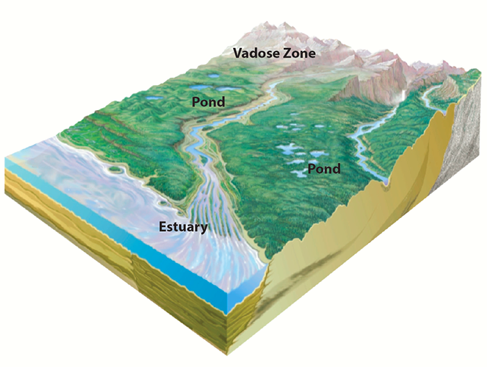
Fig. 39 Biogeochemistry occurs at many interfaces and requires a systems approach to study.#
Autochthonous Inputs#
Every system responds to various types of inputs in different ways. Autochthonous inputs into a natural system are those that originate from within the system itself. These inputs can be in the form of nutrients, energy, or other materials that are produced or generated by the system’s own biotic and abiotic processes.
In an aquatic ecosystem, autochthonous inputs may include the nutrients and organic matter produced by photosynthetic organisms like algae and aquatic plants. These inputs can support the growth of other organisms in the ecosystem, such as zooplankton and fish.
In a terrestrial ecosystem, autochthonous inputs may include the organic matter produced by plant growth and decomposition, as well as the nutrients and energy generated by the system’s own biogeochemical processes, such as nitrogen fixation by soil bacteria.
Autochthonous inputs are important for the functioning and sustainability of natural systems, as they provide the resources that support the growth and productivity of organisms within the system.
Allochthonous Inputs#
Allochthonous inputs into a natural system are those that originate from outside the system and are transported into it by external processes such as water or wind. These inputs can be in the form of nutrients, energy, or other materials that have been produced in other ecosystems or environments.
In an aquatic ecosystem, allochthonous inputs may include the organic matter and nutrients that are transported into the system by rivers or streams from surrounding terrestrial ecosystems. These inputs can support the growth of aquatic organisms and contribute to the overall productivity of the ecosystem.
In a terrestrial ecosystem, allochthonous inputs may include organic matter and nutrients that are brought into the system by animals, wind-blown dust, or water runoff from neighboring ecosystems. These inputs can affect the composition and productivity of the receiving ecosystem and can influence the interactions between different species.
Allochthonous inputs can have significant impacts on the functioning and dynamics of natural systems. For example, changes in the quantity or quality of allochthonous inputs can affect the growth and survival of organisms within the system and can alter the balance of nutrient cycling and energy flow.
In addition to their direct effects on CZ processes, autochthonous and allochthonous inputs can also interact with other factors such as climate and land use to affect the overall health and sustainability of the CZ. For example, changes in land use practices such as deforestation or agriculture can alter the balance of autochthonous and allochthonous inputs, which can have long-term impacts on soil fertility, water quality, and ecosystem productivity.
Methods to Examine Inputs#
Principal Component Analysis#
In CZ science studies there are many types of data that are collected as we see from many of the papers that we read. Many of these data are related to each other. Recognizing patterns within these data becomes very crucial to our understanding of the CZ system functions. Principal Component Analysis (PCA) is a statistical technique used to reduce the complexity of data by identifying patterns and relationships between variables. PCA is used in data analysis to condense many variables into a smaller set of variables that capture most of the important information (dimension reduction). It’s like summarizing a long article into a shorter, key point version.
Here’s a short summary of how PCA works:
Imagine a bunch of data points: These data points could represent anything. For example, data on precipitation, ET, soil type, types of trees, age of trees in a forest, etc. Each point has multiple features or variables.
Find the big picture: PCA identifies the directions of greatest variation in the data. Think of these directions as lines or planes that best fit the scattered data points.
New and improved variables: PCA creates new variables, called principal components, that align with these directions of variation. The first component captures the most variation, the second captures the remaining variation, and so on.
Less is more (sometimes): By using a smaller set of principal components, you can achieve dimensionality reduction. This means you can represent the data with fewer variables, which can be easier to analyze and visualize.
There’s a trade-off, though. PCA discards some information to create the new compressed set of variables. The key is to keep the components that hold the most important information.
PCA data are shown in biplots which combine two plots into one: a score plot and a loadings plot.
Score plot: This shows the data points themselves, projected onto the first two principal components. Each data point is represented by a dot, and its location reflects how it scores on those two components.
Loadings plot: This shows the variables used in the PCA analysis. They are represented by arrows or lines radiating from the origin. The direction of the arrow indicates how the variable is related to the principal components, and the length of the arrow reflects how much it contributes to the variation captured by that component.
By combining these two plots, a PCA biplot allows you to visualize both the relationships between the data points and the relationships between the variables. Here’s an example:

Fig. 40 Results of Principal Component Analysis of landscape predictor variables.#
Here are some key things to look for when interpreting a PCA biplot:
Grouping of data points: Do the data points cluster together, or are they spread out? Clusters suggest similar characteristics within those groups.
Direction of variable arrows: How do the variable arrows relate to each other? Are they pointing in similar directions (positive correlation), opposite directions (negative correlation), or perpendicular (no correlation)?
Length of variable arrows: The longer the arrow, the more the variable contributes to the variation captured by that principal component.
By considering these aspects of the biplot, you can gain valuable insights into the relationships between the variables and the structure of your data.
In essence, PCA is a way to simplify data by identifying the most important patterns and relationships between variables, and reducing the complexity of the data. It is a powerful tool that is used in many different fields, including sciences, engineering, humanities, and finance.
Example of PCA Application in CZS
Consider the following questions:
What was the big picture research question asked in this study?
How is the water balance affecting this stream system in the Charleston area?
How many potential water sources were identified for this stream sysem?
How was PCA used to separate the different sources and identify the more significant sources?
What was determined to be the main source of water to such stream systems?
See Principal Component Analysis (PCA) Explained Visually with Zero Math | by Casey Cheng for a nice summary of the method.
t-test#
T-tests are statistical tools used to compare the means of two groups in large sets of data. They are particularly helpful when the data comes from normally distributed populations and the variances are unknown.
There are two main types of t-tests:
One-sample t-test: This kind of test compares the mean of a single group to a hypothesized value. For instance, you might use it to see if the average precipitation in Charleston is different from the national average.
Two-sample t-test: This kind of test compares the means of two different groups. Maybe you want to see if a new fertilizer increases corn yield compared to a standard fertilizer.
Here’s the general process of how a t-test works:
Set up your hypothesis: You’ll have a null hypothesis, which is the idea you’re trying to disprove (usually that there’s no difference between the means), and an alternative hypothesis (that there is a difference).
Calculate the t-statistic: This statistic considers the difference between the group means, the variability within the groups, and the sample sizes.
Find the p-value: This value represents the probability of getting a t-statistic as extreme as the one you calculated, assuming the null hypothesis is true. Lower p-values mean there’s less chance the observed difference is due to random chance.
Interpret the results: You’ll choose a significance level (often 0.05) to decide if the p-value is small enough to reject the null hypothesis. If it is, you can conclude there’s a statistically significant difference between the means.
Example of t-test in environmental applications
Scenario: A geologist wants to investigate if there’s a difference in average lead concentration between roadside dust and soil samples collected further away from traffic in a city.
Null hypothesis (H₀): The average lead concentration in roadside dust is the same as the average lead concentration in soil further from traffic.
Alternative hypothesis (H₁): The average lead concentration in roadside dust is higher than the average lead concentration in soil further from traffic (due to traffic emissions).
Steps:
Collect data: The geologist randomly collects samples from both roadside areas and further away from traffic. They then measure the lead concentration in each sample.
Perform the t-test: Using statistical software, the geologist runs an independent samples t-test on the lead concentration data for roadside dust and soil samples.
Analyze the results: The t-test will provide a t-statistic and a p-value. Let’s say the p-value is lower than the chosen significance level (e.g., 0.05).
Interpretation: Since the p-value is statistically significant, we reject the null hypothesis. This suggests that the average lead concentration in roadside dust is statistically higher than the average lead concentration in soil further from traffic. This supports the idea that traffic emissions contribute to higher lead levels in roadside dust.
Example of t-test in critical zone sciences
Scenario: CZ researchers are interested in studying the effects of different land-use practices on soil carbon content. They collect soil samples from two different sites: one site with a forested area (Site A) and another site with an agricultural field (Site B). They measure the soil carbon content (in \(\pu{g kg-1}\) of soil) at multiple locations within each site.
The researchers want to determine if there is a significant difference in the mean soil carbon content between Site A and Site B. They can use a two-sample t-test to compare the means of the two independent samples.
Let’s assume the following data:
Site A (Forested area): Soil carbon content (\(\pu{g kg-1}\)): 28.5, 31.2, 25.7, 29.9, 27.1, 30.4 Sample size, \(n_A=6\)
Site B (Agricultural field): Soil carbon content (\(\pu{g kg-1}\)): 18.3, 20.1, 22.4, 19.7, 17.6, 21.2 Sample size, \(n_B=6\)
The researchers can perform a two-sample t-test to test the null hypothesis that there is no significant difference in the mean soil carbon content between the two sites against the alternative hypothesis that there is a significant difference.
The steps involved in performing the t-test would be:
Calculate the sample means and standard deviations for each site. Data are shown above.
Site A: Mean, \(x_A = \pu{28.8 g kg-1}\), Variance (SD), \({s_A}^2 = 4.77\)
Site B: Mean, \(x_B = \pu{19.88 g kg-1}\), Variance (SD), \({s_B}^2 = 3.61\)
Check the assumptions of normality and equal variances.
Calculate the t-statistic and degrees of freedom.
The degrees of freedom (df) for this two-sample t-test would be calculated as:
Determine the critical value from the t-distribution based on the chosen significance level (e.g., \(\alpha\) = 0.05).
Compare the calculated t-statistic with the critical value. With the t-statistic and degrees of freedom, the researchers can compare the calculated value to the critical value from the t-distribution table or use a statistical software to determine the p-value and make a decision about the null hypothesis.
Make a decision to reject or fail to reject the null hypothesis based on the comparison. For example, if you have 10 degrees of freedom and want to test at a significance level of 0.05 (α = 0.05), the critical t-value from the table is 1.812. If your calculated t-statistic is greater than this critical value, you would reject the null hypothesis.
The calculated t-statistic is greater than the critical value, the researchers can conclude that there is a significant difference in the mean soil carbon content between the forested area and the agricultural field. This result might suggest that the land-use practices (forest versus agriculture) have an impact on soil carbon content, and further investigations could be conducted to understand the underlying mechanisms.
See An Introduction to t Tests | Definitions, Formula and Examples (scribbr.com)
Stable Isotope Ratios#
Stable isotopes do not spontaneously break down to form other isotopes. Because of relative differences in masses of isotopes of an element, changes to isotopic ratios can be observed during various biogeochemical processes. Study of stable isotopes is useful in gaining better understanding in environmental and geological studies.
Stable isotopes are especially useful in elements whose isotopes have large relative mass differences. Therefore, most of the elements used for stable isotope studies have a low atomic number and atomic mass (Table 1). For isotopes with an atomic mass of greater than \(40\), the relative mass differences are too small for any measurable isotopic fractionation. Most elements used in radiometric dating have high atomic mass, and mass fractionation is not significant.
Element |
Isotope |
% |
|---|---|---|
\(\ce{H}\) |
\(\ce{^1 H}\) |
\(99.985\) |
\(\ce{H}\) |
\(\ce{^2 H}\) |
\(0.015\) |
\(\ce{C}\) |
\(\ce{^{12} C}\) |
\(98.9\) |
\(\ce{C}\) |
\(\ce{^{13} C}\) |
\(1.1\) |
\(\ce{N}\) |
\(\ce{^{14} N}\) |
\(99.63\) |
\(\ce{N}\) |
\(\ce{^{15} N}\) |
\(0.37\) |
\(\ce{O}\) |
\(\ce{^{16} O}\) |
\(99.762\) |
\(\ce{O}\) |
\(\ce{^{18} O}\) |
\(0.2\) |
Stable Isotope Fractionation#
Isotopic fractionation is the partitioning of isotopes during physical (evaporation, condensation, melting, crystallization, absorption and desorption, diffusion), chemical, or biological processes. This partitioning is proportional to the difference in the masses of the isotopes. The processes can either be equilibrium reactions, in which forward and backward reaction rates are equal for each isotope, or kinetic reactions, which are unidirectional reactions in which reaction rates are dependent on the masses of the isotopes and their vibrational energies.
Example: Stable isotope fractionation of \(\ce{H2O}\)
During evaporation of in a closed system, six isotope combinations of \(\ce{H2O}\) are possible: \(\ce{^1H2^{16}O}, \ce{^1H^2H^{16}O}, \ce{^2H2^{16}O}, \ce{^1H2^{18}O}, \ce{^1H^2H^{18}O}, \ce{^2H2^{18}O}\).
As a result of these different stable isotope combinations, the molecular masses are \(18\), \(19\), \(20\), \(20\), \(21\), and \(22\) respectively. See the conceptulizations in the figure below.

Why do stable isotopes fractionate? Isotopically lighter isotopes have higher velocities than heavier isotopes. From basic physics, kinetic energy of a particle can be calculated using the following formula:
Per Eqn. (7), isotopically lighter molecules that have higher velocities and therefore, greater amount of kinetic energy. Consider the above water example. Since the lighter molecules have greater velocities, they preferentially escape into the vapor phase resulting in enrichment of the lighter isotopes ( and ), relative to the liquid phase of water. In addition, atoms with greater mass form slightly stronger bonds, the heavier isotope is generally enriched in the more condensed phase or larger molecule.
The partitioning of stable isotopes between two substances, \(A\) and \(B\), is described by the isotopic fractionation factor, \(\alpha\). The fractionation factor is written as
where, \(R\) is ratio of heavy to light isotope abundance (e.g., \(\ce{^2 H}\)/\(\ce{^1 H}\) , \(\ce{^{18}O}\)/\(\ce{^{16}O}\) ). Generally, the isotope abundance ratio does not greatly vary in the environment, and so the fractionation factor, \(\alpha\), generally has a value close to 1. However, this value can be precisely measured and so is expressed with a precision of 4-5 decimal places. The fractionation factor depends on the temperature and can be determined either experimentally or calculated from spectroscopic data.
Example: Isotope fractionation factor
Consider the evaporation of water. We can setup the fractionation ratio and factor as follows:
We can calculate \(\alpha\) as
Since \(\ce{^{16}O}\) is enriched in the vapor phase relative to the liquid,
Conversely, \(\ce{^{18}O}\) is enriched in the liquid relative to the vapor,
Therefore, the fractionation factor is greater than 1. With increasing temperature, the fractionation factor decreases, and it becomes 1 at infinite temperature.
In Fig. 41, isotope fractionation of \(\ce{O}\) as a function of temperature during evaporation of \(\ce{H2O}\) is shown. Paleoclimatologists use \(\ce{O}\) ratios (\(\ce{^{18}O}\)/\(\ce{^{16}O}\)) from \(\ce{H2O}\) trapped in glaciers as well as the \(\ce{O}\) absorbed in the shells of marine plants and animals to measure past temperatures and rainfall. In polar ice cores, the measurement is relatively simple: less \(\ce{^{18}O}\) in the frozen water means that temperatures were cooler. In shells, the measurement is far more complicated because the biological and chemical processes that form the shells skew the \(\ce{O}\) ratio in different ways depending on temperature.
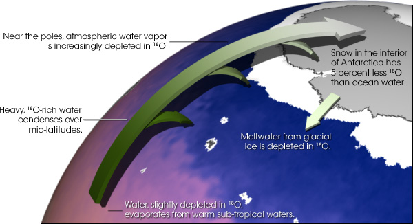
Fig. 41 Water vapor gradually loses \(\ce{^{18}O}\) as it travels from the equator to the poles. Because water molecules with heavy \(\ce{^{18}O}\) isotopes in them condense more easily than normal water molecules, air becomes progressively depleted in \(\ce{^{18}O}\) as it travels to high latitudes and becomes colder and drier. In turn, the snow that forms most glacial ice is also depleted in \(\ce{^{18}O}\). Image source: Paleoclimatology: The Oxygen Balance (nasa.gov)#
The \(\delta\) notation#
\(R\) values for environmental samples have to be compared with a fixed value (or a standard) to know if that sample is enriched or depleted compared to the standard.
Since isotopic variations between samples are very small, we express isotopic ratios using delta (\(\delta\)) notation. This value is determined by comparing the isotopic ratio (\(R\)) of a sample with that of a standard and calculated as follows:
Where the isotopic ratio, \(R\), has been defined in the previous section. Note that the ratio is multiplied by a thousand and is expressed in “parts per thousand” or permille or permil or the symbol, \(\pu{‰}\). As seen in Eqn. (9), \(R_\text{Standard}\) is required for the element of interest. Standards for most common elements of interest have been adopted worldwide for research purposes and shown in Table 2. Typically, V-SMOW (Vienna standard mean ocean water), and PDB (Pee Dee beleminite) are most commonly used for \(\ce{H}\), \(\ce{O}\), and \(\ce{C}\) ratios.
Isotope Ratio |
Standard |
\(R \times \pu{e-5}\) |
|---|---|---|
\(\ce{^2 H}\)/\(\ce{^1 H}\) |
V-SMOW |
\(15.575\) |
\(\ce{^{13} C}\)/\(\ce{^{12} C}\) |
PDB |
\(1123.75\) |
\(\ce{^{18} O}\)/\(\ce{^{16} O}\) |
V-SMOW |
\(200.52\) |
\(\ce{^{18} O}\)/\(\ce{^{16} O}\) |
PDB |
\(206.72\) |
\(\ce{^{15} N}\)/\(\ce{^{14} N}\) |
NBS-14 |
\(367.6 \) |
\(\ce{^{34} S}\)/\(\ce{^{32} S}\) |
CDT |
\(4499.4\) |
When \(\delta\) values are negative, \(R_\text{Sample} < R_\text{Standard}\) in Eqn. (9), therefore, the sample is considered to be depleted compared with the standard. Similarly, when \(\delta\) values are positive, \(R_\text{Sample} > R_\text{Standard}\), therefore, the sample is considered to be enriched compared to the standard.
Example: \(\delta\) notation
A rainwater sample collected in Boston, Massachusetts, has an \(\ce{^{18} O}\)/\(\ce{^{16} O}\) ratio of \(0.0019750\). Calculate \(\delta\) for this rainwater sample.
From Table 2, we can read the isotopic ratio of \(\ce{^{18} O}\)/\(\ce{^{16} O}\) in V-SMOW to be \(0.0020052\). Substitute values in Eqn. (9) as follows:
Since this final value is negative, the sample isotopically lighter than the standard.
Role of Organisms#
Organisms have a significant impact on the CZ. These impacts include:
Soil formation: Living organisms, especially microbes, plants, and animals, play a crucial role in the weathering of rock and the formation of soil, which is the central component of the critical zone. Organisms break down rock, cycle nutrients, and create organic matter that accumulates in the soil.
Regulating water and nutrient cycles: The roots, stems, and leaves of plants interact with the soil, water, and atmosphere to regulate the movement of water, carbon, and other nutrients through the critical zone. This cycling of water and nutrients is essential for sustaining terrestrial life.
Shaping landscape and ecosystem processes: Burrowing animals, tree roots, and other organisms physically alter the structure and composition of the critical zone, which in turn shapes landscape evolution, erosion, and the overall functioning of ecosystems.
Providing ecosystem services: The organisms in the CZ provide essential services to human society, such as food production, water filtration, and climate regulation. Disruptions to CZ organisms can degrade these important services.
The diverse array of living organisms, from microbes to large plants and animals, are intimately connected to and play a vital role in regulating the complex physical, chemical, and biological processes within the critical zone. Understanding these organism-critical zone interactions is crucial for managing natural resources and sustaining terrestrial life. See Akob and Küsel for an excellent review.
The Role of Organisms in Biogeochemistry
Read the following article: Wolves modulate soil nutrient heterogeneity and foliar nitrogen by configuring the distribution of ungulate carcasses - Bump - 2009 - Ecology
Consider the following questions:
What is the big picture research question being asked by these researchers?
What were some of the specific responses that were attributed to moose carcasses?
How were nitrogen isotopes incorporated into this study?
What are some of the positive feedback mechanisms proposed by the authors regarding the effects of wolf-killed moose carcasses?
The introduction of wolves back into wildlands is a controversial topic. What do these results say about the management of species and the functioning and stability of ecosystems?